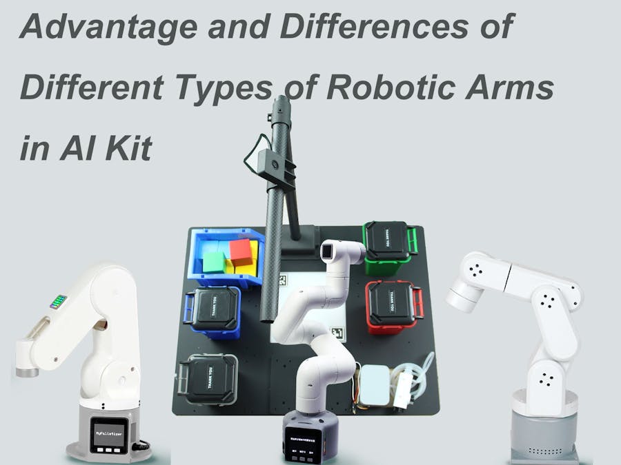
This article is primarily about introducing 3 robotic arms that are compatible with AI Kit. What are the differences between them?
If you have a robotic arm, what would you use it for? Simple control of the robotic arm to move it around? Repeat a certain trajectory? Or allow it to work in the industry to replace humans? With the advancement of technology, robots are frequently appearing around us, replacing us in dangerous jobs and serving humanity. Let's take a look at how robotic arms work in an industrial setting.
Introduction
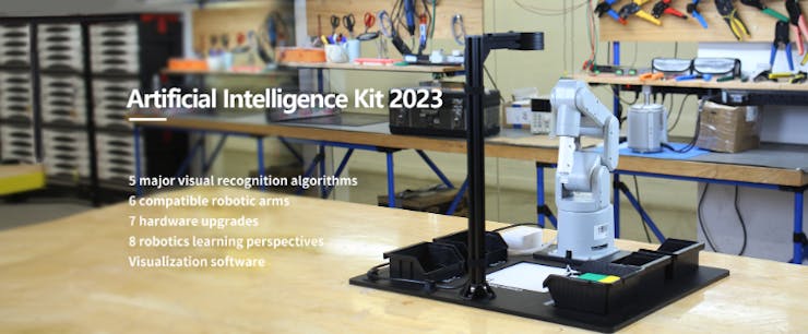
what is AI Kit?
The AI Kit is an entry-level artificial intelligence Kit that integrates vision, positioning, grasping, and automatic sorting modules. Based on the Linux system and built-in ROS with a 1:1 simulation model, the AI Kit supports the control of the robotic arm through the development of software, allowing for a quick introduction to the basics of artificial intelligence.
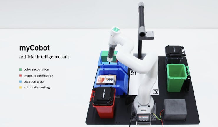
Currently, AI Kit can achieve color and image recognition, automatic postioning and sorting. This Kit is very helpful for users who are new to robotic arms and machine vision, as it allows you to quickly understand how artificial intelligence projects are built and learn more about how machine vision works with robotic arms.
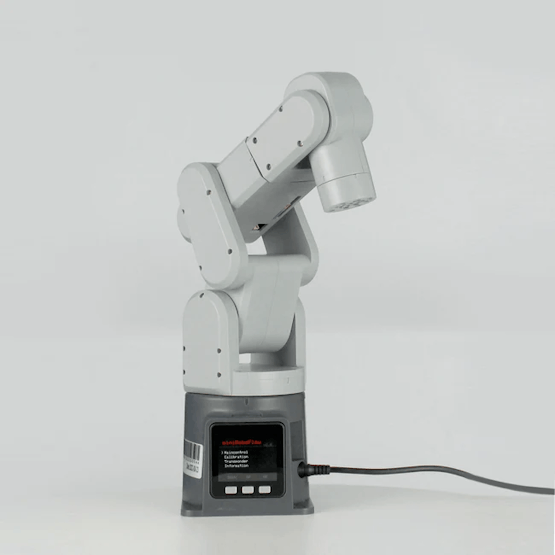
Next, let's briefly introduce the 3 robotic arms that are compatible with the AI Kit.
The AI Kit can be adapted for use with myPalletizer 260 M5Stack, myCobot 280 M5Stack and mechArm 270 M5Stack.All three robotic arms are equipped with the M5Stack-Basic and the ESP32-ATOM.
Robotic Arms
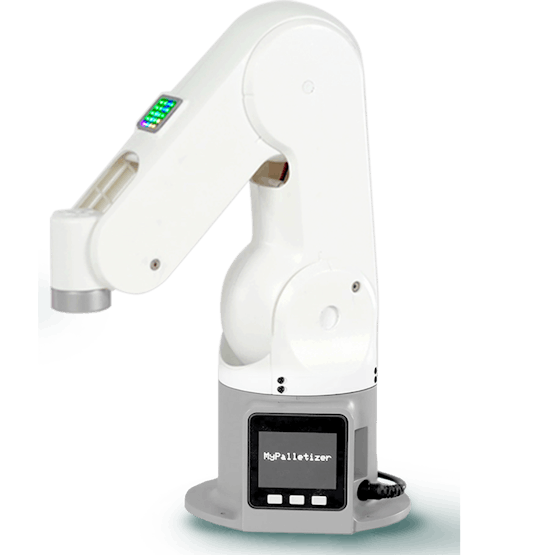
myPalletizer 260
myPalletizer260 is a lightweight 4-axis robotic arm, it is compact and easy to carry. The myPalletizer weighs 960g, has a 250g payload, and has a working radius of 260mm. It is explicitly designed for makers and educators and has rich expansion interfaces.
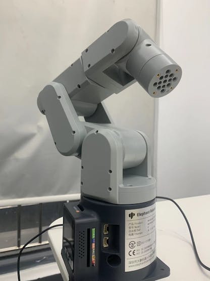
mechArm 270
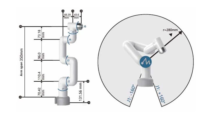
mechArm 270 is a small 6-axis robotic arm with a center-symmetrical structure (like an industrial structure). The mechArm 270 weighs 1kg with a payload of 250g, and has a working radius of 270mm. As the most compact collaborative robot, mechArm is small but powerful.
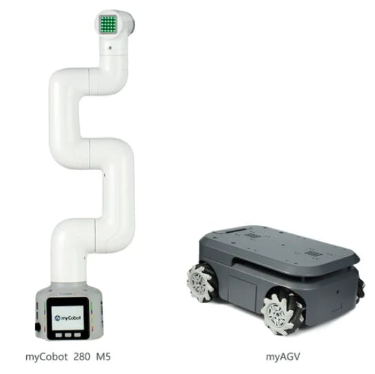
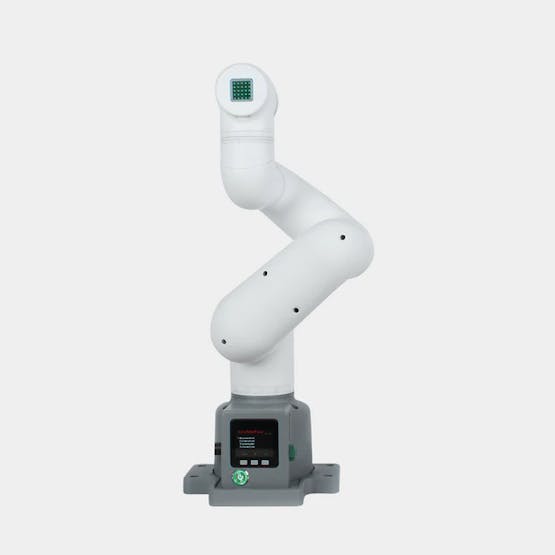
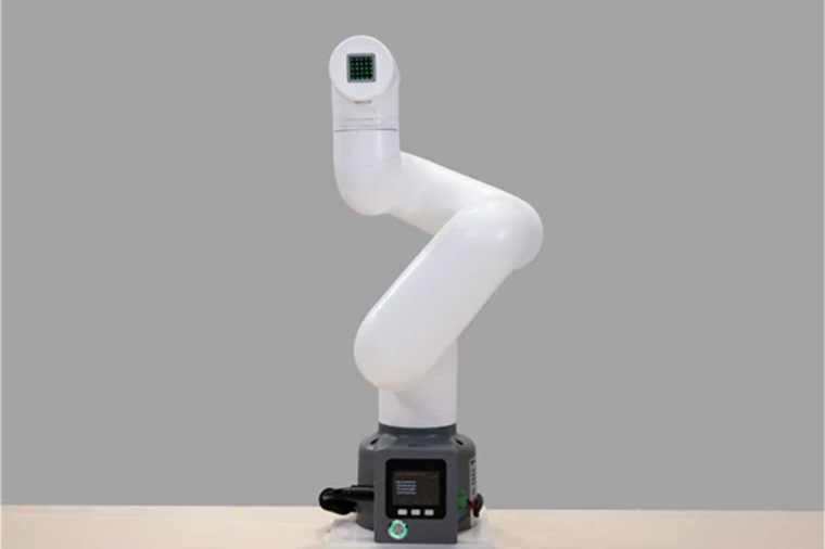
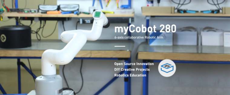
myCobot 280
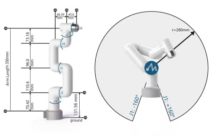
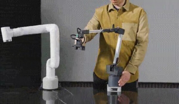
myCobot 280 is the smallest and lightest 6-axis collaborative robotic arm (UR structure) in the world, which can be customized according to user needs. The myCobot has a self-weight of 850g, an effective load of 250g, and an effective working radius of 280mm. It is small but powerful and can be used with various end effectors to adapt to various application scenarios, as well as support the development of software on multiple platforms to meet the needs of various scenarios, such as scientific research and education, smart home, and business pre R&D.

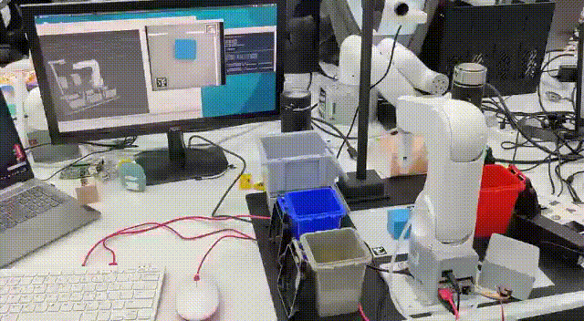
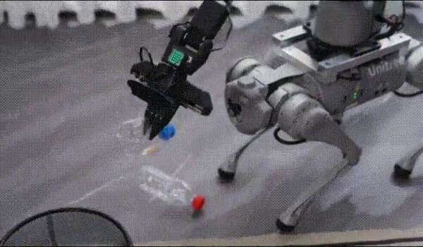
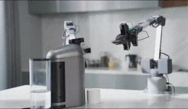
Let's watch a video to see how AI Kit works with these 3 robotic arms.
https://youtu.be/kgJeSbo9XE0
Project Description
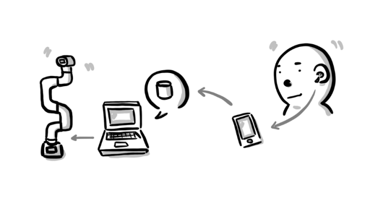
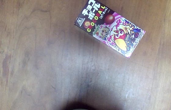
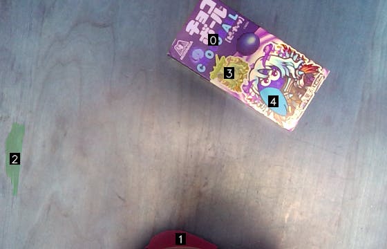
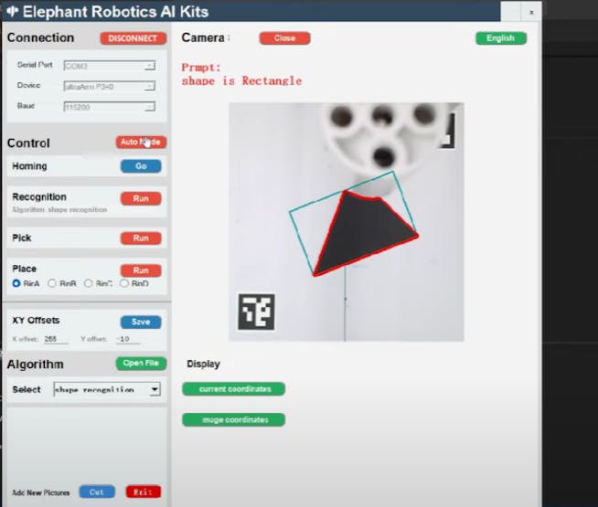
The video shows the color recognition and intelligent sorting function, as well as the image recognition and intelligent sorting function. Let's briefly introduce how AI Kit is implemented (using the example of the color recognition and intelligent sorting function).
This artificial intelligence project mainly uses two modules:
●Vision processing module
●Computation module (handles the conversion between eye to hand)
Vision processing module
OpenCV (Open Source Computer Vision) is an open-source computer vision library used to develop computer vision applications. OpenCV includes a large number of functions and algorithms for image processing, video analysis, deep learning based object detection and recognition, and more.
We use OpenCV to process images. The video from the camera is processed to obtain information from the video such as color, image, and the plane coordinates (x, y) in the video. The obtained information is then passed to the processor for further processing.
Here is part of the code to process the image (colour recognition)
# detect cube color
def color_detect(self, img):
# set the arrangement of color'HSV
x = y = 0
gs_img = cv2.GaussianBlur(img, (3, 3), 0) # Gaussian blur
# transfrom the img to model of gray
hsv = cv2.cvtColor(gs_img, cv2.COLOR_BGR2HSV)
for mycolor, item in self.HSV.items():
redLower = np.array(item[0])
redUpper = np.array(item[1])
# wipe off all color expect color in range
mask = cv2.inRange(hsv, item[0], item[1])
# a etching operation on a picture to remove edge roughness
erosion = cv2.erode(mask, np.ones((1, 1), np.uint8), iterations=2)
# the image for expansion operation, its role is to deepen the color depth in the picture
dilation = cv2.dilate(erosion, np.ones(
(1, 1), np.uint8), iterations=2)
# adds pixels to the image
target = cv2.bitwise_and(img, img, mask=dilation)
# the filtered image is transformed into a binary image and placed in binary
ret, binary = cv2.threshold(dilation, 127, 255, cv2.THRESH_BINARY)
# get the contour coordinates of the image, where contours is the coordinate value, here only the contour is detected
contours, hierarchy = cv2.findContours(
dilation, cv2.RETR_EXTERNAL, cv2.CHAIN_APPROX_SIMPLE)
if len(contours) > 0:
# do something about misidentification
boxes = [
box
for box in [cv2.boundingRect(c) for c in contours]
if min(img.shape[0], img.shape[1]) / 10
< min(box[2], box[3])
< min(img.shape[0], img.shape[1]) / 1
]
if boxes:
for box in boxes:
x, y, w, h = box
# find the largest object that fits the requirements
c = max(contours, key=cv2.contourArea)
# get the lower left and upper right points of the positioning object
x, y, w, h = cv2.boundingRect(c)
# locate the target by drawing rectangle
cv2.rectangle(img, (x, y), (x+w, y+h), (153, 153, 0), 2)
# calculate the rectangle center
x, y = (x*2+w)/2, (y*2+h)/2
# calculate the real coordinates of mycobot relative to the target
if mycolor == "red":
self.color = 0
elif mycolor == "green":
self.color = 1
elif mycolor == "cyan" or mycolor == "blue":
self.color = 2
else:
self.color = 3
if abs(x) + abs(y) > 0:
return x, y
else:
return None
Just obtaining image information is not enough, we must process the obtained data and pass it on to the robotic arm to execute commands. This is where the computation module comes in.
Computation module
NumPy (Numerical Python) is an open-source Python library mainly used for mathematical calculations. NumPy provides many functions and algorithms for scientific calculations, including matrix operations, linear algebra, random number generation, Fourier transform, and more. We need to process the coordinates on the image and convert them to real coordinates, a specialized term called eye to hand. We use Python and the NumPy computation library to calculate our coordinates and send them to the robotic arm to perform sorting.
Here is part of the code for the computation.
while cv2.waitKey(1) < 0:
# read camera
_, frame = cap.read()
# deal img
frame = detect.transform_frame(frame)
if _init_ > 0:
_init_ -= 1
continue
# calculate the parameters of camera clipping
if init_num < 20:
if detect.get_calculate_params(frame) is None:
cv2.imshow("figure", frame)
continue
else:
x1, x2, y1, y2 = detect.get_calculate_params(frame)
detect.draw_marker(frame, x1, y1)
detect.draw_marker(frame, x2, y2)
detect.sum_x1 += x1
detect.sum_x2 += x2
detect.sum_y1 += y1
detect.sum_y2 += y2
init_num += 1
continue
elif init_num == 20:
detect.set_cut_params(
(detect.sum_x1)/20.0,
(detect.sum_y1)/20.0,
(detect.sum_x2)/20.0,
(detect.sum_y2)/20.0,
)
detect.sum_x1 = detect.sum_x2 = detect.sum_y1 = detect.sum_y2 = 0
init_num += 1
continue
# calculate params of the coords between cube and mycobot
if nparams < 10:
if detect.get_calculate_params(frame) is None:
cv2.imshow("figure", frame)
continue
else:
x1, x2, y1, y2 = detect.get_calculate_params(frame)
detect.draw_marker(frame, x1, y1)
detect.draw_marker(frame, x2, y2)
detect.sum_x1 += x1
detect.sum_x2 += x2
detect.sum_y1 += y1
detect.sum_y2 += y2
nparams += 1
continue
elif nparams == 10:
nparams += 1
# calculate and set params of calculating real coord between cube and mycobot
detect.set_params(
(detect.sum_x1+detect.sum_x2)/20.0,
(detect.sum_y1+detect.sum_y2)/20.0,
abs(detect.sum_x1-detect.sum_x2)/10.0 +
abs(detect.sum_y1-detect.sum_y2)/10.0
)
print ("ok")
continue
# get detect result
detect_result = detect.color_detect(frame)
if detect_result is None:
cv2.imshow("figure", frame)
continue
else:
x, y = detect_result
# calculate real coord between cube and mycobot
real_x, real_y = detect.get_position(x, y)
if num == 20:
detect.pub_marker(real_sx/20.0/1000.0, real_sy/20.0/1000.0)
detect.decide_move(real_sx/20.0, real_sy/20.0, detect.color)
num = real_sx = real_sy = 0
else:
num += 1
real_sy += real_y
real_sx += real_x
The AI Kit project is open source and can be found on GitHub.
Difference
After comparing the video, content, and code of the program, it appears that the 3 robotic arms have the same framework and only need minor modifications to the data to run successfully.
There are roughly two main differences between these 3 robotic arms.
One is comparing the 4- and 6-axis robotic arms in terms of their practical differences in use (comparing myPalletizer to mechArm/myCobot).
Let's look at a comparison between a 4-axis robotic arm and a 6-axis robotic arm.
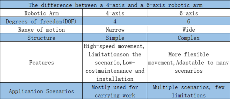
From the video, we can see that both the 4-axis and 6-axis robotic arms have a sufficient range of motion in the AI Kit's work area. The main difference between them is that myPalletizer has a simple and quick start process with only 4 joints in motion, allowing it to efficiently and steadily perform tasks, while myCobot requires 6 joints, two more than myPalletizer, resulting in more calculations in the program and a longer start time (in small scenarios).
In summary, when the scene is fixed, we can consider the working range of the robotic arm as the first priority when choosing a robotic arm. Among the robotic arms that meet the working range, efficiency and stability will be necessary conditions. If there is an industrial scene similar to our AI Kit, a 4-axis robotic arm will be the first choice. Of course, a 6-axis robotic arm can operate in a larger space and can perform more complex movements. They can rotate in space, while a 4-axis robotic arm cannot do this. Therefore, 6-axis robotic arms are generally more suitable for industrial applications that require precise operation and complex movement.
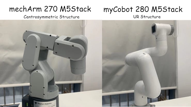
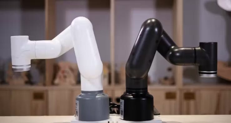
The second thing is that both are 6-axis robotic arms, and their main difference is the structure. mechArm is a centralized symmetrical structure robotic arm, and myCobot is a UR structure collaborative robotic arm. We can compare the differences between these two structures in actual application scenarios.
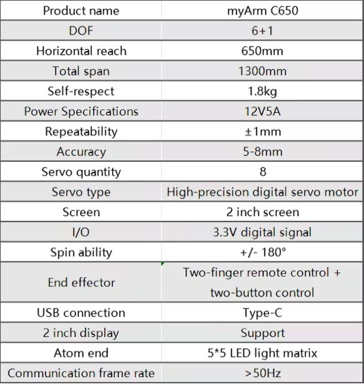
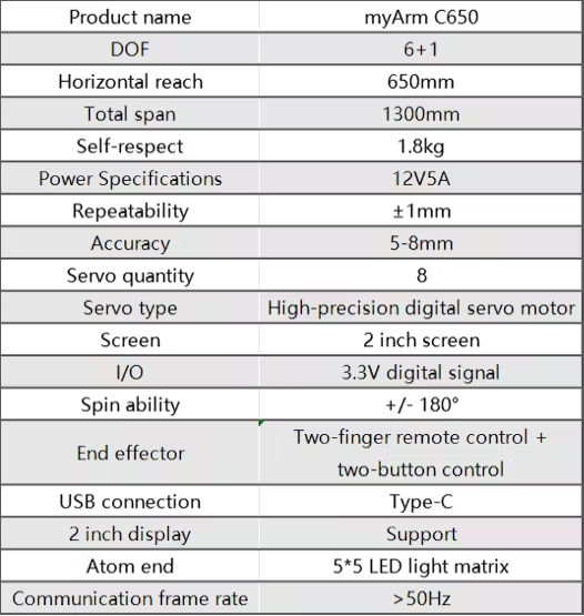
Here are the specifications of the two robotic arms.
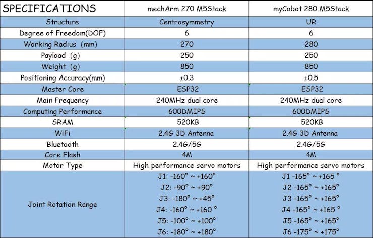
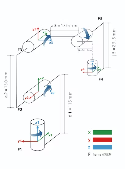
The difference in structure between these two leads to a difference in their range of motion. Taking mechArm as an example, the centrally symmetrical structure of the robotic arm is composed of 3 pairs of opposing joints, with the movement direction of each pair of joints being opposite. This type of robotic arm has good balance and can offset the torque between joints, keeping the arm stable.
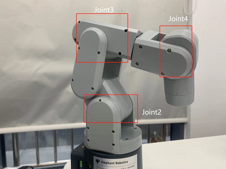
Shown in the video, mechArm is also relatively stable in operation.
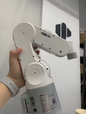
You may now question, is myCobot not useful then? Of course not, the UR structure robot arm is more flexible and can achieve a larger range of motion, suitable for larger application scenarios. myCobot's more important point is that it is a collaborative robot arm, it has good human-robot interaction ability and can collaborate with humans for work. 6-axis collaborative robot arms are usually used in logistics and assembly work on production lines, as well as in medical, research, and education fields.
Summary
As stated at the beginning, the difference between these 3 robotic arms included in the AI Kit is essentially how to choose a suitable robotic arm to use. If you are choosing a robotic arm for a specific application, you will need to take into consideration factors such as the working radius of the arm, the environment in which it will be used, and the load capacity of the arm.
If you are looking to learn about robotic arm technology, you can choose a mainstream robotic arm currently available on the market to learn from. MyPalletizer is designed based on a palletizing robotic arm, mainly used for palletizing and handling goods on pallets. mechArm is designed based on a mainstream industrial robotic arm, which has a special structure that keeps the arm stable during operation. myCobot is designed based on a collaborative robotic arm, which is a popular arm structure in recent years, capable of working with humans and providing human strength and precision.
That's all for this post, if you like this post, please leave us a comment and a like!
We have published an article detailing the differences between mechArm and myCobot.Please click on the link if you are interested in learning more.


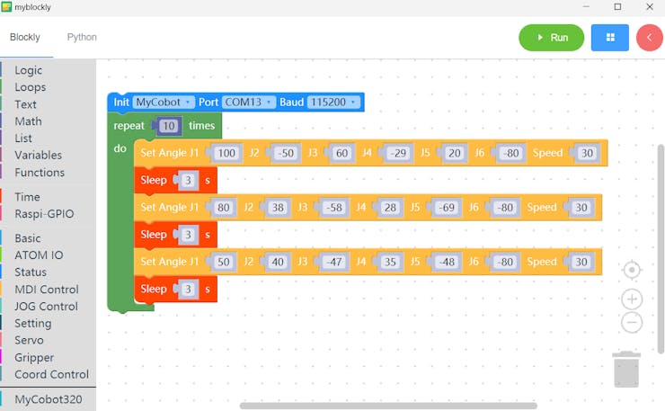


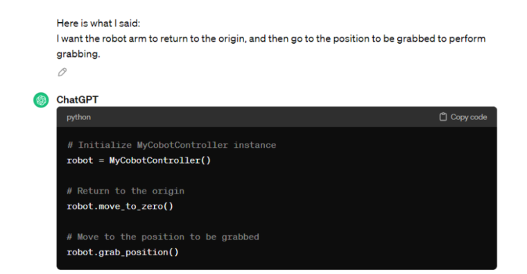
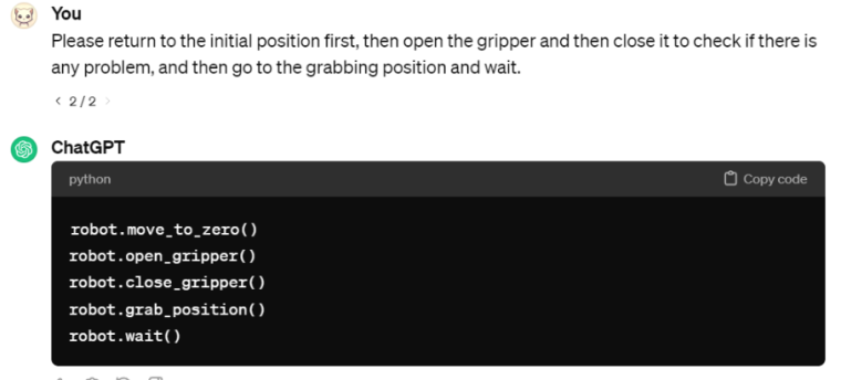 Copy the generated code and run it.
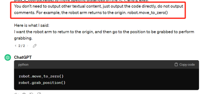